The code offered here compiles programs written in a simple imperative language down to the one-instruction Subleq language. For example, sum.imp:
include(`defs.m4')
# sum 1 to i

LABELS

printStr([Enter i ])
input(i)

label(startL)
add(sum, sum, i)
decr(i)
condJump(i, outL)
goto(startL)

label(outL)
printStr([Sum: ])
println(sum)

HALT

# --------- data -----------
NAMES
i:0   sum:0   0
can be compiled into the Subleq triplets in sum.tri:
0 0 3
69 -3 6
110 -3 9
116 -3 12
101 -3 15
114 -3 18
32 -3 21
105 -3 24
  :  # many lines not shown
0 0 0
0 0 0
-1 0 1
-10 32 44
0 0 0
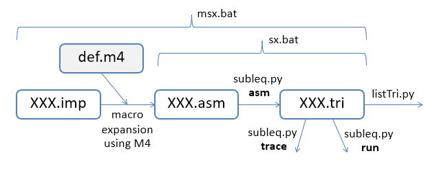
The various steps in the compilation:
The fact that such a compiler can be written shows (informally) that although Subleq only supports a single instruction it's still capable of executing a full range of algorithms (i.e. it is Turing complete).
The compiler is not a recursive descent parser based on BNF syntax rules. Instead, I've reached back to a technique from the very early days of computing – text macros. I've employed the venerable macro language m4, developed by Brian Kernighan and Dennis Ritchie for UNIX in the mid 1970s, but still a part of GNU/Linux.
A macro specifies how a string can be replaced by another, perhaps with various arguments instantiated. For example,
define(ENDFILE -1)
causes all occurrences of ENDFILE to be replaced by -1 in the file being processed.
The popularity of macro processing back in the "Jurassic" era of programming is due to its simple and efficient approach to language extension, especially when the target language is syntactically simple. For instance, it's a popular approach for adding features to Lisp-like languages, and LaTeX is written in the TeX macro language.
I chose macro processing since Subleq is very assembly-like, and replacing imperative features by snippets of Subleq code makes it clear that Subleq is a fully capable programming language. The macros are relatively short, and less complicated than a recursive descent compiler.
On the downside are the traditional problems with text macros – the lack of variable scoping, poor support for debugging, compile-time vs. runtime bindings, and the absence of syntactic information. I'll describe these issues in detail in later examples.
Subleq is an OISC (One Instruction Set Computer) language, meaning that the (virtual) machine only supports one instruction, but the language is still capable of implementing any algorithm possible in more conventional languages. It's perhaps the most popular of an increasingly large group of OISC languages, many of which are listed at the Esolangs website.
The Subleq instruction is "SUBtract and branch if Less-than or EQual to zero", which operates upon three adjacent memory addresses, a triplet I'll call (A, B, C). The operation can be defined in pseudo-code as:
def subleq(PC) =
  A = mem[PC]; B = mem[PC+1]; C = mem[PC+2]
  mem[B] = mem[B] - mem[A]
  if mem[B] <= 0:
    PC = C
  else:
    PC = PC + 3
PC is the program counter, which accesses the linear memory data structure mem[].
The value stored in memory address A is subtracted from the value stored in memory address B, with the result written back into B. If the result is less than or equal to zero, then execution jumps to memory address C; otherwise it continues onto the next triplet.
cycle1.tri executes forever, jumping between the first and third triplets while evaluating the data in the second triplet:
3 4 6
7 7 7
3 4 0
The execution is illustrated below:
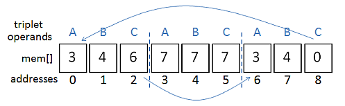
The first triplet subtracts the 7 stored in address 3 from the 7 in address 4. The 0 result is stored back in address 4, overwriting the 7, and computation jumps to address 6, the start of the third triplet. This triplet also subtracts the contents of address 3 from address 4, (0 - 7) resulting in -7 being stored in address 4 and execution jumping back to the first triplet. This to-and-fro between the triplets continues indefinitely, while the data in address 4 keeps decreasing.
Since cycle1.tri doesn't output anything, the best approach is to run the Subleq interpreter (subleq.py) in trace mode:
> python subleq.py trace cycle1.tri
-------- Execution ----------
         pc: (  a,   b,   c)   mem[a]  mem[b]

          0: (  3,   4,   6)      7       7
          6: (  3,   4,   0)      7       0
          0: (  3,   4,   6)      7      -7
          6: (  3,   4,   0)      7     -14
          0: (  3,   4,   6)      7     -21
          6: (  3,   4,   0)      7     -28
          0: (  3,   4,   6)      7     -35
          6: (  3,   4,   0)      7     -42
          0: (  3,   4,   6)      7     -49
          6: (  3,   4,   0)      7     -56
          0: (  3,   4,   6)      7     -63
                 :
                 :
The jumping between the first and third triplets (starting at address 0 and 6 respectively) is quite apparent, and the last column shows that the contents of address 4 keeps decreasing in steps of 7.
It's also useful to call listTri.py to show how the triplets are stored in memory:
> python listTri.py cycle1.tr

  0: (  3,   4,   6)
  3: (  7,   7,   7)
  6: (  3,   4,   0)
The interpreter is closely based on subleq.py available from the Esolangs website. I've made a number of changes, including the removal of the class structuring, the addition of extra output modes and an input mode, and a few cosmetic alterations.
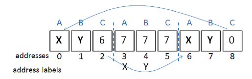
As detailed on the Subleq website, the interpreter allows memory addresses to be labeled. A program augmented in this way is stored in an ".asm" file, and is compiled down to plain Subleq triplets saved to a ".tri" file. For example, we can rewrite the cyclic example as cycle2.asm:
X Y 6
X:7 Y:7 7
X Y 0
This code labels addresses 3 and 4 as "X" and "Y", and uses those labels in the first and third triplets instead of addresses. Aside from those labeling changes, the program's execution will be unchanged, as depicted in:
Calling subleq.py with the asm option compiles this program down to its basic form:
> python subleq.py asm cycle2.asm
Saving subleq instruction to cycle2.tri
The fact that the generated triplets are the same as before can be checked by calling listTri.py:
> python listTri.py cycle2.tri

  0: (  3,   4,   6)
  3: (  7,   7,   7)
  6: (  3,   4,   0)
Yet another version of this program is in cycle3.asm:
# infinite cycling between two triples

Y -1    # print Y
X Y 6
X Y 0

# ------ data --------
X:7 Y:7 0    # must be three per line
".asm" files can include comments (beginning with '#'). Also, the first line of the program uses address -1 to print the integer value stored in memory address Y. The 'triplet' hasn't a C term, which is taken by the interpreter to mean that it should always jump to the next triplet. In addition, I've moved the data (the X and Y 'variables') to more clearly separate the program's code and data. Note that Subleq triplets always require three values, so the final unused 0 on the data line is required.
A visualization of the program:
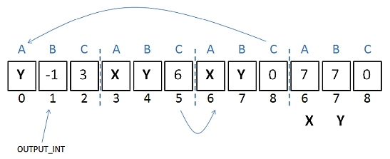
Since the second triplet always jumps to the third triplet, I could have coded it as "X Y" rather than "X Y 6", but making the jump explicit seems clearer.
The inclusion of the print operation means that the program can be usefully executed with subleq.py's run option:
> python subleq.py asm cycle3.asm
Saving subleq instruction to cycle3.tri

> python subleq.py run cycle3.tri
7 -7 -21 -35 -49 -63 -77 -91 -105 -119 -133 -147 -161 -175 -189
-203 -217 -231 -245 -259 -273 -287 -301 -315 ...
This combination of "asm" and "run" is so common that I've packaged it up in a batch file, sx.bat:
> sx.bat cycle3.asm
Compiling cycle3.asm...
Saving subleq instruction to cycle3.tri

Running cycle3.tri...
7 -7 -21 -35 -49 -63 -77 -91 -105 -119 -133 -147 ...
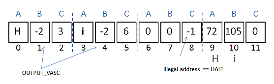
H -2     # print var's value as ASCII
i -2
0 0 -1   # halt

# ------ data --------
H:72 i:105 0
This time the output operand is -2, which means that the values stored in the memory addresses for 'H' and 'i' are printed as ASCII values.
The third triplet employs the -1 halt code. The triplet subtracts the value stored in address 0 from itself and jumps to the address -1 (since the result of subtracting a number from itself is always 0). When the PC of the virtual machine is set to a negative address, execution terminates.
A visualization of the program:
The program's compilation and execution:
> sx hi1.asm
Compiling hi1.asm...
Saving subleq instruction to hi1.tri

Running hi1.tri...
Hi
The -1 and -2 output modes print out the data stored at the supplied addresses. For example, H -2 prints the data stored in the address labeled as 'H'. In the diagram above, 'H' is address 9, and the printed data is the ASCII version of 72.
A useful simplification when printing ASCII is to remove one level of redirection by utilizing the -3 output mode. For example, hi2.asm:
72 -3     # print value as ASCII
105 -3
0 0 -1   # halt
This approach means that there's no need for a 'data' section in the program (e.g. as in hi1.asm).
The program's compilation and execution:
> sx hi2.asm
Compiling hi2.asm...
Saving subleq instruction to hi2.tri

Running hi2.tri...
Hi
Addition is a little tricky since the Subleq instruction only offers subtraction. add1.asm assumes that a and b contain the values being added, and uses a third variable, t to build an intermediate result before storing it in res:
a t     # t = 0 - a
b t     # t = -a - b
t res   # res = 0 - -(a + b)
res -1  # print res
0 0 -1  # halt

# ------- vars ----------
res:0 a:60 b:7
t:0 0 0
The program's compilation and execution:
> sx add1.asm
Compiling add1.asm...
Saving subleq instruction to add1.tri

Running add1.tri...
67
>
add2.asm employs the -4 input mode to read in values for a and b:
97 -3    # print 'a'
a -4     # input int
98 -3    # print 'b'
b -4     # input int

a t
b t
t res
res  -1
0 0 -1

# ------- vars ----------
res:0 a:0 b:0
t:0 0 0
The program's compilation and execution:
> sx add2.asm
Compiling add2.asm...
Saving subleq instruction to add2.tri

Running add2.tri...
a>> 45
b>> 55
100
The ">>" before the user's input is part of the input operation, but the 'a' and 'b' before the ">>"s are printed ASCII.
At the start of this post, I defined Subleq as:
def subleq(PC) =
  A = mem[PC]; B = mem[PC+1]; C = mem[PC+2]
  mem[B] = mem[B] - mem[A]
  if mem[B] <= 0:
    PC = C
  else:
    PC = PC + 3
It's now possible to compare this with the virtual machine implemented by subleq.py in run():
def run(mem, isTrace=False):
  if isTrace:
    print("-------- Execution ----------")
  pc = 0
  if isTrace:
    print(f"\t pc: (  a,   b,   c)   mem[a]  mem[b]\n")
  while pc >= 0:
    a = mem[pc]
    b = mem[pc+1]
    c = mem[pc+2]
    if isTrace:
      memA = memStr(a)
      memB = memStr(b)
      print(f"\t{pc:3d}: ({a:3d}, {b:3d}, {c:3d})
                         {memA:>4}    {memB:>4}")
    result = 0
    if b >= 0:
      result = mem[b] - mem[a]
      mem[b] = result
    elif b == OUTPUT_INT:  # -1
      # print mem[a] value as an integer
      print( printInt(mem[a]), end='')

    elif b == OUTPUT_VASC:  # -2
      # print mem[a] value as ASCII char
      print( printAscii(mem[a]), end='')

    elif b == OUTPUT_ASC:  # -3
      # print address a as ASCII char
      print( printAscii(a), end='')

    elif b == INPUT_PORT:   # -4
      mem[a] = int(input(">> "))

    pc = c if result <= 0 else pc + 3
                          # next triple
The code is complicated by the trace mode, and the if-tests dealing with the three output modes (B == -1, -2, or -3) and the input mode (B == -4).
m4 is a general-purpose macro processor designed by Brian Kernighan and Dennis Ritchie for UNIX in 1977. Despite its age, the original 6-page technical report is still a great introduction. In more modern times, the version used most widely is GNU m4, and its manual is excellent. Also, probably because of its age, there's a lot of other good quality documentation, including:
m4 is an extension of an an earlier macro processor, m3, also written by Dennis Ritchie. A version of this tool is implemented from scratch in the classic textbook, Software Tools by Brian Kernighan and P.J. Plauger, although I'd recommend that an interested reader search for the later edition, Software Tools in Pascal, which benefits from using Pascal rather than Ratfor (in particular, Pascal offers recursion). The book is currently available for borrowing from the Internet Archive, and the source code has been preserved by Shuo Chen on Github.
m4 is a standard tool on GNU/Linux machines, and versions for other platforms can be obtained from the GNU website. However, my preference on Windows is the copy included with Gow, a minimal installer of about 130 UNIX tools pre-compiled as native Win32 binaries:
> gow --list
Available executables:
  awk, basename, bash, bc, bison, bunzip2, bzip2,
  bzip2recover, cat, chgrp, chmod, chown, chroot,
  cksum, clear, cp, cs, csplit, curl, cut, dc, dd,
  df, diff, diff3, dirname, dos2unix, du, egrep,
  env, expand, expr, factor, fgrep, flex, fmt, fold,
  gawk, gfind, gow, grep, gsar,   gsort, gzip, head,
  hostid, hostname, id, indent, install, join, jwhois,
  less, lesskey, ln, ls, m4, make, md5sum, mkdir, mkfifo,
  mknod, mv, nano, ncftp, ngrep, nl, od, pageant, paste,
  patch, pathchk, plink, pr, printenv, printf, pscp, psftp,
  putty, puttygen, pwd, rm, rmdir, scp, sdiff, sed, seq,
  sftp, sha1sum, shar, sleep, split, ssh, su, sum, sync,
  tac, tail, tar, tee, test, touch, tr, uname, unexpand,
  uniq, unix2dos, unlink, unrar, unshar, uudecode,
  uuencode, vim, wc, wget, whereis, which, whoami, xargs,
  yes, zip
>
Gow includes GNU m4 v.1.4.13, while the current release has reached 1.4.21 (as of May 2026), but I've not had any problems with the earlier version.
examples.m4 contains seven macros, of increasing complexity:
define(`GREETING', `Hello, World!')dnl
GREETING

define(`SQUARE', `(($1) * ($1))')dnl
SQUARE(5)

define(`DEBUG', `1')dnl
ifdef(`DEBUG', `Debugging is ON', `Debugging is OFF')

define(`DOUBLE', `eval(($1) * 2)')dnl
DOUBLE(7)

define(`FACT',
  `ifelse($1, 0, 1, `eval($1 * FACT(eval($1-1)))')')dnl
FACT(5)

define(`forloop',
  `ifelse($2, $3, `$4',
    `$4`'define(`$1', eval(($2)+1))`'
    forloop(`$1', eval(($2)+1), $3, `$4')')')dnl
define(`i', 1)dnl
forloop(`i', 1, 5, `Item i
')
define(macroName, macroText) creates a named macro, and when that name is encountered in the input is replaced by the associated text.
examples.m4 utilizes eval() and ifelse(), two built-in commands. eval() evaluates its argument using arithmetic and logical operations similar to those in C. ifelse(text1, text2, eqText, neqText) tests if text1 and text2 are equal; if they are then eqText is expanded, otherwise neqText is processed.
The macro processing produces:
> m4 -d examples.m4
# examples.m4

Hello, World!

((5) * (5))

Debugging is ON

14

120

Item 1
Item 2
Item 3
Item 4
Item 5
>
m4's "-d" option turns on a range of debugging checks.
It's more common to place macro definitions in a separate file. Consider myDefs.m4:
divert(-1)

changequote([,])

define([N], 50)
define([inc], [$1 = $1 + 1])
define([M], [[N]])

define([avg], [eval(($1 + $2)/2)])

define([sqr1], [$1 * $1])
define([sqr2], [($1) * ($1)])

divert
I'm working with a foreign language keyboard which uses the backquote key (`) to switch between languages. This makes '`' less than ideal as a way of quoting text, so the call to changequote() switches the quoting to square brackets.
These macros are included at the start of defsTest.txt:
include(`myDefs.m4')

average1 = avg(4, 5)
average2 = avg(x, 5)

a = sqr1(5)
b = sqr1(5+2)
c = sqr2(5+2)
When the file is macro expanded, the results are:
> m4 -d defsTest.txt

average1 = 4
average2 = m4:defsTest.txt:4:
   bad expression in eval (bad input): (x + 5)/2

a = 5 * 5
b = 5+2 * 5+2
c = (5+2) * (5+2)
The error message for "average2 = avg(x, 5)" shows that eval() requires both arguments to avg() to be numerical at expansion time.
The two versions of the squaring macro illustrate how macro processor works with text tokens, not at the syntactic level. The first macro generates "5+2 * 5+2" which according to usual arithmetic means 5 + (2*5) + 2, or 17. The precedence of math operations is expressed in a recursive descent parser by manipulating a syntax tree reflecting BNF rules. However, this knowledge is unavailable to the token replacement mechanism used by macros. The simplest fix is to include brackets in the text expansion, as in the second version of the macro.
Another source of confusion with m4 is when macros are expanded, which is partly controlled by the use of quoting around the macro name and the macro text. A good rule-of-thumb is to always quote both in a define(), but matters often become more complex when a define() appears inside another define() (as in the forloop macro given above in examples.m4).
Quoting is also an issue with how macros are called. The two macros in quotes.m4 are defined conventionally, with their names and text both quoted. However, we must also think about the quoting of the arguments passed to those macros. Three common cases are shown:
divert(-1)

traceon(`active', `show')

define(`active', `ACT, IVE')
define(`show', `$1 $1')

divert dnl

show(active)       # ACT ACT
#
show(`active')     # ACT, IVE ACT, IVE
#
show(``active'')   # active active
traceon() turns on a detailed tracing of how and when the macros are expanded:
> m4 -d quotes.m4

m4trace: -2- active -> `ACT, IVE'
m4trace: -1- show(`ACT', `IVE') -> `ACT ACT'
ACT ACT       # ACT ACT
#
m4trace: -1- show(`active') -> `active active'
m4trace: -1- active -> `ACT, IVE'
ACT, IVE m4trace: -1- active -> `ACT, IVE'
ACT, IVE     # ACT, IVE ACT, IVE
#
m4trace: -1- show(``active'') -> ``active' `active''
active active   # active active
The numbers between dashes indicating the ordering and depth of the expansions.
The first call to show() shows the effect of not quoting its input argument, meaning that the argument will be expanded before the show() call. Therefore, show() receives two tokens `ACT' and `IVE', and it duplicates the first, producing `ACT' and `ACT'.
The second call to show() delays the expansion of its input argument until after show() has been expanded. Therefore, the expansion will be of `active active', producing two copies of `ACT, IVE'.
The third call uses double quoting to force show()'s argument to be treated as text, and never be expanded.
The diagram at the top of this post shows how m4 is employed as a preprocessor to convert programs written in a simple imperative style into the ".asm" assembler-like language. The high-level code is stored in an ".imp" file, and GNU m4 imports macros from defs.m4 to rewrite it.
The "Bottom-up Building" title of this post refers to how I developed the macros in defs.m4 – I started with simple macros like toZero(), assign(), add(), and ifCond(), then used some of those to build more complex macros such as abs() and multiply().
add3.imp illustrates many of the basic macros:
include(`defs.m4')

LABELS

print(a)
println(b)

assign(res, a)
println(res)

toZero(res)
add(res, a, b)  # res = a + b
print(res)

HALT

# --- data ---
NAMES
res:0 a:60 b:7
The expanded text is written to "add3.asm":
0 0   # needed for labels

a -1    # print a
b -1    # print b
NL -1

_tmp1 _tmp1     # res = a
a _tmp1
res res
_tmp1 res
res -1    # print res
NL -1

res res
_tmp1 _tmp1     # res = a + b
a _tmp1
b _tmp1     # _tmp1 = -a - b
res res
_tmp1 res
res -1    # print res

zero zero -1   # halt

# --- data ---
_tmp1:0  _tmp2:0  _tmp3:0
_tmp4:0  _tmp5:0  _tmp6:0
#
minus1:-1  zero:0  one:1
NL:-10   space:32  comma:44

res:0 a:60 b:7
addSub.m4 illustrates the macros printStr(), input(), and sub(), while hi3.m4 and hi4.m4 employ printA() and printAA() for printing ASCII characters.
The following are a sample of the macros in defs.m4:
define([NAMES], [_tmp1:0  _tmp2:0  _tmp3:0
_tmp4:0  _tmp5:0  _tmp6:0
#
minus1:-1  zero:0  one:1
NL:-10   space:32  comma:44
])


define([print], [$1 -1    # print $1])


define([assign], [_tmp1 _tmp1     # $1 = $2
$2 _tmp1
$1 $1
_tmp1 $1 ])


define([toZero], [$1 $1])


define([add], [_tmp1 _tmp1     # $1 = $2 + $3
$2 _tmp1
$3 _tmp1     # _tmp1 = -$2 - $3
$1 $1
_tmp1 $1 ])


define([HALT], [zero zero -1   # halt])
NAMES is a collection of temporary variables and constants used by many of the other macros.
The biggest problem with using predefined variables such as _tmp1 is scope. A macro is not a function, where the scope of its variables is limited to the function. As add3.asm above illustrates, the temporary variables added by a macro's expansion are global to the entire program. This means that it's possible that the changes to a variable in one macro could inadvertently affect that variable's use in a different macro. For instance, _tmp1 is utilized by both assign() and add() in add3.asm.
A good coding style that combats this situation is to always reinitialize variables at the start of a macro, as in assign() and add(). Sadly, this doesn't always solve the problem since a more complex macro may expand another macro within itself. In that case, reinitialization of a variable in the inner macro might change the same-named variable in the outer macro.
As a rather feeble solution, the NAMES macro includes six temporary variables. If a macro author feels that using _tmp1 might cause a conflict, he/she can always switch to _tmp2 with the hope that the problem will be avoided.
The batch file msx.bat calls the m4 processor followed by subleq.py. Essentially, the script contains:
set AS=%~nS1%.asm
set TS=%~nS1%.tri

m4 -d %S1% > %AS%
python subleq.py asm %AS%
python subleq.py run %TS%
It's also possible to process a ".imp" file individually, by directly calling m4 -d XXX.imp > XXX.asm. This is good practice when testing a new macro since the resulting expansion can be examined before involving the Subleq interpreter.
Control flow is implemented using four macros: condJump(), goto(), label(), and LABELS, as seen in if.imp:
LABELS

printStr([Enter c ])
input(c)
condJump(c, thenL)  # if c <= 0 goto thenL
printStr([Pos])     # ELSE branch
goto(haltL)
label(thenL)        # THEN branch
printStr([Neg])
goto(haltL)

L_HALT(haltL)

# --- data ---
NAMES
c:0 0 0
If c is less than or equal to 0 then 'Neg" is printed, otherwise 'Pos' is output. The program's compilation and execution:
> msx if.imp
Expanding Macros...
Compiling if.asm...
Saving subleq instruction to if.tri

Running if.tri...
Enter c >> 5
Pos
The relevant macro definitions in defs.m4:
define([condJump], [zero $1 $2   # if $1<=0 jump to $2])

define([goto], [zero zero $1     # goto address $1])

define([label], [$1:$1 0         # label $1])

define([LABELS], [0 0   # needed for labels])
zero is one of the predefined variables in NAMES, and has the value 0 as you might expect.
The trickiest macro here is LABELS, which adds the triplet (0, 0, 3) to the start of the ".asm" file. It's utilized by label() which expands to the triplet (X, 0, X+3) stored at memory address X, which can then be used as the destination for goto(X).
The need for LABELS arises because the (X, 0, X+3) triplet will be executed. The calculation mem[B] = mem[B] - mem[A] writes a negative number into mem[0], and LABELS places a 'dummy' triplet at that address to prevent this assignment changing anything important.
sum.imp uses these macros to implement a loop that sums the integers between 1 and i:
LABELS

printStr([Enter i ])
input(i)

label(startL)
add(sum, sum, i)
decr(i)
condJump(i, outL)
goto(startL)

label(outL)
printStr([Sum: ])
println(sum)

HALT

# --------- data -----------
NAMES
i:0   sum:0   0
The program's compilation and execution:
> msx sum.imp
Expanding Macros...
Compiling sum.asm...
Saving subleq instruction to sum.tri

Running sum.tri...
Enter i >> 5
Sum: 15
fib.imp calculates the first n values in the Fibonacci sequence:
> msx fib.imp
Expanding Macros...
Compiling fib.asm...
Saving subleq instruction to fib.tri

Running fib.tri...
Enter n >> 8
1 1 2 3 5 8 13 21
Occasionally, it's clearer to express a jump as a triplet rather than as a goto, as in cycle.imp:
LABELS

label(startL)
print(Y)
X Y nextL

label(nextL)
X Y startL

HALT

# ------ data --------
NAMES
X:7 Y:7 0
It's quite clear that we could simplify this program by removing the nextL label.
The examples on the Subleq page at the Esolangs website are fairly easy to understand except for the "Hello, World" program. It's difficulty is partly due to the low-level language, but is also compounded by the use of two clever programming tricks – sentinels and dynamic addressing.
The code can be written as in hello1.imp:
# print from START+1 address to END

LABELS

assign(_ptr, START)
incr(_ptr)      # move to start of text

label(_startL)
assign(_pCh, _ptr)

printA(_pCh:0)  # a dynamic address
   # this will print the value at mem[_ptr]

incr(_ptr)      # move through addresses

# loop while (_ptr < END) or (_ptr - END + 1) <= 0
sub(t, _ptr, END)
incr(t)
condJump(t, _startL)
nl()

HALT

# ------------ data ---------------
NAMES
_ptr:0 t:0 0
# _pCh NOT defined here

0 0 START:START
72 101 108      # "Hello, World!"
108 111 44
32 87 111
114 108 100
33  END:END 0
The sentinels are the memory addresses START:START and END:END which surround the ASCII data representing "Hello, World!". This labeling style means that the memory address stores its own address. START is used to initialize _ptr, which is then incremented in a loop until it reaches END.
The code's use of dynamic addressing can be seen in the lines:
assign(_pCh, _ptr)
printA(_pCh:0)
The _ptr value (a memory address between START and END) is stored in mem[_pCh] by assign(), and printA() prints the ASCII value stored in that _ptr memory address. Therefore, each time that printA() is called it accesses a different memory address (between START and END) and prints the ASCII value stored there.
The ".asm" code for these two lines in hello1.asm is:
_tmp1 _tmp1     # _pCh = _ptr
_ptr _tmp1
_pCh _pCh
_tmp1 _pCh

_pCh:0 -2    # printA(_pCh:0)
The printA line in the ".tri" file can also be examined with python listTri hello1.tri:
33: ( 0, -2, 36) ; print ascii mem[0]
along with the data block for the "Hello, World!" string:
 87: (  0,   0,  89)   # START == 89
 90: ( 72, 101, 108)   #  H  e  l
 93: (108, 111,  44)   #  l  o  ,
 96: ( 32,  87, 111)   # ' ' W  o
 99: (114, 108, 100)   #  r  l  d
102: ( 33, 103,   0)   #  !  END == 103
If the ".tri" code is executed in trace mode then we can observe how address 33 of the printA triplet changes:
> python subleq.py trace hello1.tri
    :
33: ( 90,  -2,  36)     72  --   # print H stored in addr 90
    :
33: ( 91,  -2,  36)    101  --   # e
    :
33: ( 92,  -2,  36)    108  --   # l
    :
Although dynamic addressing is complicated, it's also very versatile. For example, it's the core of how GOSUB/RETURN is implemented, as explained below.
A macro becomes much harder to implement correctly if it calls other macros, mainly due to the variable scoping issue and the difficulty of understanding how quoting affects nested macro expansion. The three version of the multiply() macro in multiply.imp illustrate what I mean:
LABELS

printStr([Enter a and b:])
nl()
input(a)
input(b)

# --------- mult1 -------------
# b causes inf loop
mult1(t, a, 3)      # was a*b, but do a*3 instead
printStr([mult1: ])
println(t)

# --------- mult2 -------------

printStr([mult2: ])
mult2(t, a, b)
  # if b is negative then it's treated like 0
println(t)

# --------- multiply() -------------

printStr([multiply: ])
multiply(t, a, b)
println(t)

HALT

# --- data ---
NAMES
a:3 b:7 t:7
s:0 b1:0 0
mult1() and mult2() are incorrect. For instance, consider the following run:
> msx multiply.imp
Expanding Macros...
Compiling multiply.asm...
Saving subleq instruction to multiply.tri

Running multiply.tri...
Enter a and b:
>> 5
>> -7
mult1: 15
mult2: 0
multiply: -35
Thankfully, multiply() is correct, but its use of abs(), a macro for calculating an absolute value, made it very difficult to successfully debug.
mult1() returns 15 due to my editing of the multiply.imp program, replacing b by 3. If the variable isn't commented out then macro expansion goes into a loop. The 'easiest' way to see this is by adding some debugging prints to the _mul_loop() macro that mult1() employs:
define([mult1],   # $1 = $2 * $3
[toZero($1)
_mul_loop($1, $2, $3)
])

define([_mul_loop],
[ifelse($3, 0, [],
[add($1, $1, $2)
printStr([v:])  # debugging
print($1)
print($2)
println($3)
_mul_loop($1, $2, eval($3 - 1)) ])])
Calling m4 -d multiply.imp creates an unending stream of macro expansions:
   :
118  -3    # printAA 'v'
58  -3    # printAA ':'

t -1    # print t
a -1    # print a
-352 -1    # print -352
NL -1
_tmp1 _tmp1     # t = t + a
t _tmp1
a _tmp1     # _tmp1 = -t - a
t t
_tmp1 t
118  -3    # printAA 'v'
58  -3    # printAA ':'

t -1    # print t
a -1    # print a
-353 -1    # print -353
NL -1
_tmp1 _tmp1     # t = t + a
  :
The expansion of println($3) (the printing of the b argument) shows that its memory address has become negative, and is busy decreasing (e.g. it changes from -252 to -253 in the snippet above). This is due to the repeated failure of the ifelse() test of $3 == 0 since $3 doesn't have an assigned value at macro expansion time.
mult2() works correctly when the b value is positive, but returns 0 if b is negative. It's definition:
define([mult2],  # $1 = $2 * $3
[genLabel([_loopL])dnl
genLabel([_endL])dnl
toZero($1)
assign(_tmp3, $3)   # since changed
label([_loopL])
condJump(_tmp3, [_endL])
add($1, $1, $2)
decr(_tmp3)
goto([_loopL])
label([_endL])
])
In an early version of mult2(), $3 was decremented inside its multiplication loop, and the loop exited when $3 == 0. Since macro expansion replaces $3 by b, it meant that mult2() decremented b, leaving it equal to 0. Unfortunately, this approach led to the failure of the subsequent call to multiply() in multiply.imp since it reused b which was now 0. This problem was caused by thinking that the argument passed to mult2() was copied into it, but of course mult2() is not a function, and b is globally visible throughout multiply.imp. The current version of mult2() (shown above) starts by assigning $3 to _tmp3, and condJump(_tmp3, [_endL]) jumps out of the multiplication loop when _tmp3 <= 0.
Although, this test works correctly when $3 (b) is positive, the loop exits occurs immediately when the $3 argument is negative. This means that the result in $1 is never changed from 0.
The multiply() macro utilizes the same approach as mult2(), but starts by obtaining the absolute values of both inputs, and their signs (positive or negative) before entering its multiplication loop. After the result has been calculated, the signs data is used to negate the final answer if necessary.
The abs() macro is essentially just a single if-test, but complicated by the use of genLabel() to generate unique label names:
define([abs],
# abs($1, $2, $3) ; $2 = 1 or -1,  $3 = |$1|
[genLabel([_negAbsL])dnl
genLabel([_endAbsL])dnl
assign($3, $1)
condJump($1, [_negAbsL])
# positive case
assign($2, one)   # 1 means positive
goto([_endAbsL])
label([_negAbsL])
negate($3)
assign($2, minus1)   # -1 means negative
label([_endAbsL])
])
genLabel() utilizes a global _tempCnt integer to generate a label of the form symXX, where XX is the current counter value.
multiply() has three parts – the calls to abs() to normalize the inputs, the multiplication loop, and the use of the signs information to set the correct sign of the result:
define([multiply],
# mult3()  $1 = $2 * $3
[genLabel([_loopM3L])dnl
genLabel([_endM3L])dnl
abs($2, _tmp3, _tmp4)   # sign, abs
abs($3, _tmp5, _tmp6)

toZero($1)   # multiplication loop
label([_loopM3L])
condJump(_tmp6, [_endM3L])
add($1, $1, _tmp4)
decr(_tmp6)
goto([_loopM3L])
label([_endM3L])

genLabel([_negsign1L])dnl
genLabel([_endsign1L])dnl
genLabel([_negsign2L])dnl
genLabel([_endsign2L])dnl
condJump(_tmp3, [_negsign1L])   # set result sign
goto([_endsign1L])
label([_negsign1L])
negate($1)
label([_endsign1L])

condJump(_tmp5, [_negsign2L])
goto([_endsign2L])
label([_negsign2L])
negate($1)
label([_endsign2L])
])
Although the code utilizes unique label names, this was not enough to prevent the label expansion going 'wrong' in an earlier version of multiply(). The error was found by testing abs() separately (see absTest.imp, and by adding calls to printStr() and print() as a rudimentary way to narrow in on the problem. It turned out to be that abs() and multiply() both used the variable _endL which instead of being expanded to different symXX labels were expanding to the same name.
The lesson of all of these problem is that the lack of variable scoping in macro processing tools like m4 is a major issue. This is hardly news, and one of the development strands in macro languages since the 1970s are hygienic macros.
fact.imp uses the multiply() macro to implement factorial. For example:
> msx fact.imp
Expanding Macros...
Compiling fact.asm...
Saving subleq instruction to fact.tri
Running fact.tri...
Enter i >> 5
Fact: 120

> msx fact.imp
Expanding Macros...
Compiling fact.asm...
Saving subleq instruction to fact.tri
Running fact.tri...
Enter i >> 7
Fact: 5040
gosubTest.imp implements a function that prints its input argument and returns:
LABELS

goto(mainL)

# --------- f(i) function ------------
label(fL)

println(retTo)
assign(retJmp, retTo)

printStr([In f: ])
println(i)

goto(retJmp:0)  # return using dynamic goto


# --------- main ------------
label(mainL)

printAA(i)
input(i)
assign(retTo, retHere)
goto(fL)   # call f(i)
label(retHere)

printStr([Back])

HALT

# ----------------------------
NAMES
i:0  retTo:0 0
GOSUB is implemented as a goto() jump to a label at the start of the function code. The more interesting part is the coding of RETURN which utilizes a label in the main body (retHere in this example), a variable that passes that return address to the function (retTo), and a dynamic goto (the line goto(retJmp:0)). That line is translated into zero zero retJmp:0 in the ".asm" file, which makes retJmp the address of the third term in that triplet. Therefore the earlier assignment, assign(retJmp, retTo), has the effect of writing the retTo value into that memory cell. This is the return address in the main body, and so sets up the return.
The dynamic nature of goto(retJmp:0) is more obvious in sumG.imp which calls a sum() function three times from different lines in the main code. The program's execution:
> msx sumG.imp
Expanding Macros...
Compiling sumG.asm...
Saving subleq instruction to sumG.tri

Running sumG.tri...
i = 5
sum = 15
i = 7
sum = 28
i = 9
sum = 45
factG.imp is another example, with the main code calling fact() twice:
> msx factG.imp
Expanding Macros...
Compiling factG.asm...
Saving subleq instruction to factG.tri

Running factG.tri...
i = 5
fact = 120
i = 7
fact = 5040
This GOSUB/RETURN implementation employs a single dynamic goto in each function to set the return address to the caller. This means that a function cannot be recursive, since a new call to the function will overwrite any earlier return address setting.
Support for recursion would require me to implement a call stack to keep track of the various instances of the function, which is a level of complexity I'd rather avoid.
The dynamic goto used here is more commonly called the assigned goto – the goto jumps to a statement label (or line number) that's stored in (assigned to) an integer variable. It was a common feature in early programming languages, such as FORTRAN, and was only removed from that language in Fortran 95.
It's worth distinguishing the assigned goto from the standard form which was fairly quickly replaced by structured programming constructs. The assigned goto's slower disappearance reflects it's usefulness for certain types of advanced programming such as dispatch tables, finite state machines, Python-style generators, continuations, backtracking, and coroutines. Indeed, it's still present in C/C++ via GCC's labels-as-values extension. It's also never left assembly language programming where it's known as an indirect branch or computed jump.
Although I've demonstrated that an imperative-like language can be layered over Subleq by adding macros, it's arguable that this approach has a scalability problem due to variable scoping, the lack of syntactic support for the high-level language, the complexity of quoting, compile time macro expansion vs. runtime execution, and the paucity of debugging tools.
Nevertheless, with careful development, it is possible to use macros to build a rich language. One impressive example is the m4 BASIC to C converter written by Peter van Eerten, whose macros are collected in basic.m4.
Consider the factorial BASIC program in fact.m4b:
FUNC fact(int n)
  INTEGER res, i
  IF n < 1 THEN
    LET res = 0
  ELSE
    LET res = 1
    FOR i = 2 TO n
      LET res = res * i
    NEXT
  ENDIF
  RETURN res
ENDFUNC

REM -------------------
INTEGER res, n
LET n = 5
LET res = fact(n)
PRINT n, res FORMAT "Factorial %ld == %ld\n"
It's translated to C using:
m4 -d basic.m4 fact.m4b > fact.c
The result, fact.c (after some reformatting):
#include <stdlib.h>
#include <stdio.h>
#include <unistd.h>
#include <string.h>
#include <math.h>
#include <time.h>
#include <sys/ioctl.h>
#include <gc.h>
#define _MEMTYPE char
#define _maxdigit 32
#define _bufsize 256
int
main (int argc, char *argv[])
{
  int RETVAL;
  unsigned char _ptr = 0;
  char *_sbuf[256] = { NULL };
  GC_INIT ();
  srandom ((unsigned int) time (NULL));

  int fact (int n)
  {
    long res = 0;
    long i = 0;
    if (n < 1) {
      res = 0;
    }
    else {
      res = 1;
      for (i = 2; i <= n; i += 1) {
	res = res * i;
      }
    }
    return (res + 0);
  }

  /* ------------------------------------------ */
  long res = 0;
  long n = 0;
  n = 5;
  res = fact (n);
  fprintf (stdout, "Factorial %ld == %ld\n", n, res);
  return (0);
}
The includes of sys/ioctl.h and gc.h can be deleted, along with the calls to GC_INIT() and srandom(), which allows the program to be immediately compiled and run on most platforms:
> gcc -o fact fact.c -lm

> fact
Factorial 5 == 120