
The Python code described here focuses on the area of Game Theory involving simultaneous games, such as the Prisoner's Dilemma and Rock, Paper, Scissors. Each game is played multiple times between multiple participants to determine and then visualize the pure and mixed-strategy Nash Equilibria (NEs).
I developed these programs as part of a course based on William Spaniel's "Game Theory 101: The Complete Textbook", and his excellent videos on Youtube. Indeed, most of my examples come from his videos and/or textbook. If you're unfamiliar with simultaneous games then I highly recommend chapters 1 and 3 and the corresponding videos, numbered #1 to #15 and #27 to #37.
The four programs -- sim22.py, sim33.py, sim44.py, and simNN.py -- are named after the size of the payoff matrix they can process (sim22.py for 2x2, sim33.py for 3x3, sim44.py for 4x4, and simNN.py for NxN, where N > 2).
The standard 2x2 payoff matrix for the Prisoner's Dilemma:

The first player's preferences (to stay "quiet" or "confess") appear in the rows, and the other player's preferences are in the columns. The first player's payoffs are listed first for each outcome, and the second player's are second. For example, if the first player keeps quiet and the second player confesses, then the game ends in the top right payoff pair with the first player receiving twelve months in jail and the second player walking free.
sim22.py can use this payoff matrix to find NEs for the game:
> python sim22.py pd.txt
Reading pd.txt
Building 2 x 2 payoff...
Labels: ['Prisoners Dilemma', 'quiet', 'confess']
Payoffs: [[(-1, -1), (-12, 0)], [(0, -12), (-8, -8)]]
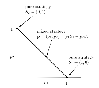
The results are displayed as a 1-simplex of barycentric coordinates spread out along a diagonal representing the probabilities of selecting the two preferences (S1 and S2):
The simplex generated for the pd.txt payoff matrix is:
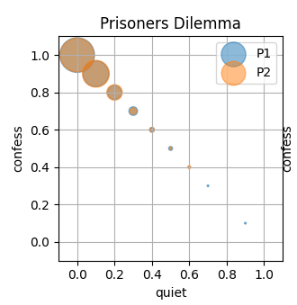
The first and second players' preferences (labeled as P1 and P2) are shown on the same graph, and in this case coincide. P1 and P2 favor an almost pure strategy NE of (confess, confess). This matches the NE calculated in Spaniel's video Game Theory 101, #2.
The actual output of sim22.py is a window containing ten copies of the 1-simplex. Repeated game play is used to accommodate the random way in which the code converges upon a NE. There may be several NEs for a given matrix, and by generating multiple graphs, we give the program a chance to converge on different results depending on how the random process develops. The benefits of this approach can be seen when processing the payoff matrix for "Battle of the Sexes":

Calling:
> python sim22.py battle27.txt
Reading battle27.txt
Building 2 x 2 payoff...
Labels: ['Battle of the Sexes', 'ballet', 'boxing']
Payoffs: [[(1, 4), (0, 0)], [(0, 0), (4, 1)]]
The ten graphs consist of multiple copies of two NEs:
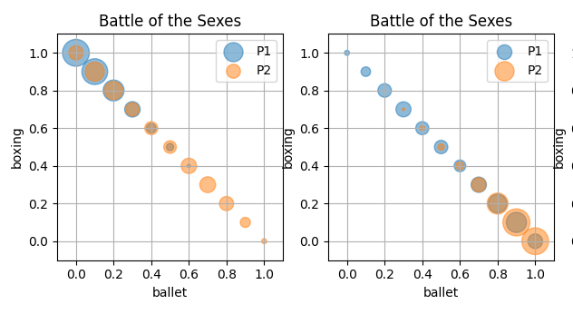
As Spaniel explains in the Game Theory 101, #27 video there are two pure NE for this matrix: (boxing, boxing) and (ballet, ballet). There's also a mixed strategy which sadly doesn't appear as a separate graph in the output of sim22.py. Instead it affects the distributions of the probabilities in the 'pure' results so that the choices for P2 in the left-hand graph, and P1 in right-hand graph, aren't concentrated solely on boxing and ballet. This issue appears in a number of the examples, when a mixed strategy NE has a lower payoff than pure strategies, causing the simulation to not converge completely upon a pure NE.
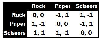
The standard example of a 3x3 payoff matrix is for the "Rock, Paper, Scissors" game:
Calling:
> python sim33.py rps36.txt
Reading rps36.txt
Building 3 x 3 payoff...
Labels: ['RPS', 'rock', 'paper', 'scissors']
Payoffs: [[(0, 0), (-1, 1), (1, -1)], [(1, -1), (0, 0), (-1, 1)], [(-1, 1), (1, -1), (0, 0)]]
The result is a 2-simplex visualization of barycentric coordinates inside an equilateral triangle, where each vertex is one of the payoff preferences:
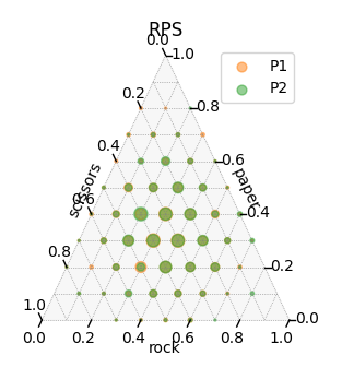
This indicates that the best strategy is (1/3, 1/3, 1/3), a mixed Nash equilibrium. For more details, see Spaniel's videos Game Theory 101, #34 and #36.
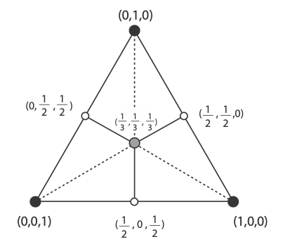
The 2-simplex allow us to treat a barycentric coordinate as a point linked by 'springs' of fractional strengths to the three vertices. For example, if the three springs have equal values (1/3, 1/3, 1/3) then the point will be located at the center of gravity of the triangle. A few other values are shown in the diagram below:
Note that whereas the other programs only utilize Matplotlib, sim33.py also depends on the python-ternary module, which needs to be installed separately.
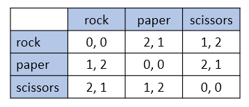
A more visually interesting nonzero-sum variant of RPS is fictitious play with the payoff matrix:
The sim33.py call and result:
> python sim33.py fictious.txt
Reading fictious.txt
Building 3 x 3 payoff...
Labels: ['RPS', 'rock', 'paper', 'scissors']
Payoffs: [[(0, 0), (2, 1), (1, 2)], [(1, 2), (0, 0), (2, 1)], [(2, 1), (1, 2), (0, 0)]]
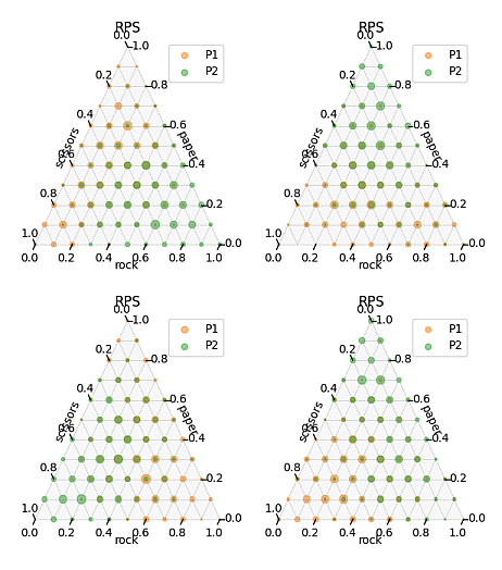
Fictitious play doesn't always converge to a NE, which is reflected in the spread of points inside the simplex, and the number of different visualizations.
A typical payoff matrix using four preferences is the "Units in a Battle" game discussed in Spaniel's video Game Theory 101, #6:
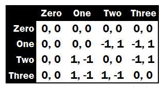
Two generals each have three units and are preparing for an upcoming battle. Each can choose to send any number of units (up to 3) to the fight or none at all. The side with more troops wins the battle, but the fight will be a draw if there are equal forces. Victory is worth 1 point; defeat is rewarded with -1. If the two sides draw or at least one side sends no units, then both sides earn 0.
One way to visualize a 3-simplex is as a tetrahedron, allocating a preference to each vertex:
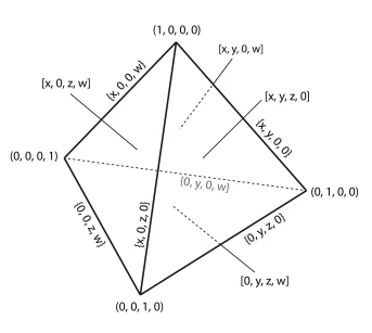
This approach is taken by sim44.py by using the 3D charting features of Matplotlib. For instance:
> python sim44.py generals.txt
Reading generals.txt
Building 4 x 4 payoff...
Labels: ['Units in a Battle', 'Pass', 'One', 'Two', 'Three']
Payoffs: [[(0, 0), (0, 0), (0, 0), (0, 0)], [(0, 0), (0, 0), (-1, 1), (-1, 1)],
[(0, 0), (1, -1), (0, 0), (-1, 1)], [(0, 0), (1, -1), (1, -1), (0, 0)]]
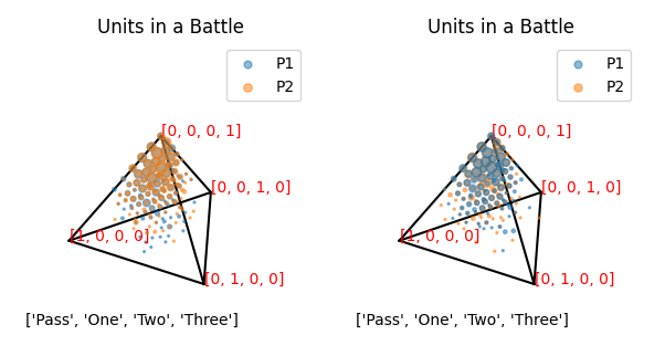
Although there appears to be two distinct results generated across the ten games, they're actually identical since the 3D alpha blending of the orange and blue points sometimes favors one color over the other. In fat, there's a single NE at (Three, Three). However, Spaniel shows that there are four possible NEs, at (Pass, Pass), (Pass, Three), (Three, Pass), and (Three, Three). I admit to being unclear why the other three equilibria never appear in the sim44.py results.
simNN.py visualizes payoff matrices with three or more preferences by utilizing Wachspress coordinates which position generalized barycentric coordinates inside a convex polygon. Each payoff preference is assigned to a vertex, and a point p inside the polygon is located based on weights related to the triangle areas specified by the point and pairs of adjacent vertices:
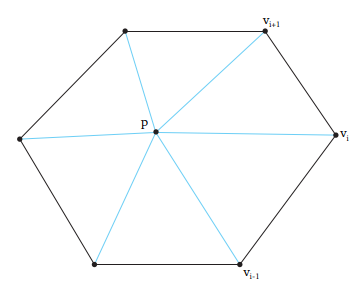
Weights for p are defined relative to every vertex i:

where A(a,b,c) is the triangle area formed by the points (a,b,c).
These weights are normalized relative to the entire area of the polygon:

where n is the number of vertices.
Note that Wachspress coordinates on the boundary of the polygon are undefined because of division by zero. Also, simNN.py employs a regular polygon of N sides as the simplex, where N is the number of preferences in the loaded payoff matrix. For example, the visualization of the 4x4 matrix for the "Units in a Battle" game from the last section utilizes a square:
> python simNN.py generals.txt
Reading generals.txt
Building 4 x 4 payoff...
Labels: ['Units in a Battle', 'Pass', 'One', 'Two', 'Three']
Payoffs: [[(0, 0), (0, 0), (0, 0), (0, 0)], [(0, 0), (0, 0), (-1, 1), (-1, 1)],
[(0, 0), (1, -1), (0, 0), (-1, 1)], [(0, 0), (1, -1), (1, -1), (0, 0)]]
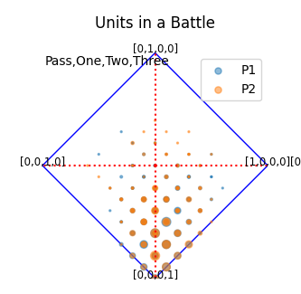
Although simNN.py's output is less 'beautiful' than sim22.py and sim33.py's for 3x3 and 4x4 payoff matrices, it does let the user click on a point, causing its barycentric coordinate to be printed to standard output. This is quite useful for larger polygons where the values for interior points are harder to determine. For instance, clicking a large dot near the "Three" vertex in the diagram above, produces bary coords: [0.16, 0.04, 0.15, 0.65].
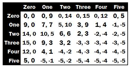
In section 1.2.2 of his textbook, Spaniel develops a 6x6 payoff matrix for duopolistic competition:
This can be processed by simNN.py:
> python simNN.py duoComp6.txt
Reading duoComp6.txt
Building 6 x 6 payoff...
Labels: ['Duo Comp', 'Zero', 'One', 'Two', 'Three', 'Four', 'Five']
Payoffs: [[(0, 0), (0, 9), (0, 14), (0, 15), (0, 12), (0, 5)],
[(9, 0), (7, 7), (5, 10), (3, 9), (1, 4), (-1, -5)],
[(14, 0), (10, 5), (6, 6), (2, 3), (-2, -4), (-2, -5)],
[(15, 0), (9, 3), (3, 2), (-3, -3), (-3, -4), (-3, -5)],
[(12, 0), (4, 1), (-4, -2), (-4, -3), (-4, -4), (-4, -5)],
[(5, 0), (-5, -1), (-5, -2), (-5, -4), (-5, -4), (-5, -5)]]
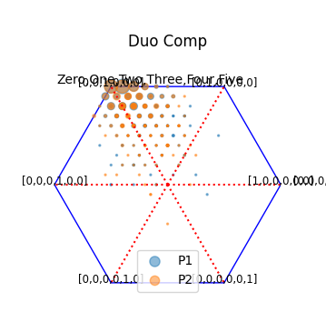
Although the output is a bit messy, it confirms Spaniel's calculation that the NE occurs at (Two, Two). (The "Zero" preference is drawn on the positive x-axis, and subsequent preferences are placed counter-clockwise around the origin.)
A more serious problem is that the code takes over one minute to generate the ten graphs. This is a consequence of gtUtils.py implementing large n-dimensional arrays as nested lists. For example, the six preferences here require two arrays for each simplex. An obvious improvement would be to switch to Numpy arrays.
sim22.py, sim33.py, sim44.py, and simNN.py utilize the same code for playing simultaneous games based on a payoff matrix by calling functions in gtUtils.py and instantiating multiple Player objects.
Initially, each preference is equally likely to be chosen, but their weights are updated at the end of each round of games. If the total score for a preference exceeds the average score for the round then the preference's weight is incremented, or decremented if it falls below. So, as multiple rounds (usually about 700) are played out, the weights are adjusted to favor the preferences producing the best score. Also, this process is carried out twice for each player to find the 'best' preferences when the player goes first, and when it goes second.
For example, consider the processing of a 2x2 payoff matrix: at the end of one round, out of 10 players, 4 may favor preference 1, and 6 favor preference 2 (when playing first). This is recorded in a 10x10 stratsP1 array by adding 1 to the stratsP1[4][6] cell.
By the end of all the rounds, stratsP1 (and stratsP2 when the player is second) are converted into a list of barycentric coordinates with associated sizes. For instance, if stratsP1[4][6] contains 20 then the resulting coordinate will be (4/10, 6/10) with point size 20. The division by the number of players ensures that the two floats add up to 1.